
Analytical geometry studies geometry with algebra. Also referred to as Cartesian geometry, the branch was first conceived by renowned French philosopher and mathematician Rene Descartes. Analytical or coordinate geometry is essentially an extension of conventional geometric reasoning that introduces the coordinate system and employs analytical or algebraic methods for studying shapes and structures.
Analytic geometry is a core topic in both elementary & applied mathematics. You will have to contend with loads of assignments on it during your first & second years and, if you choose to, through your senior years & beyond. Cracking the toughest problems& scoring good grades in analytical geometry problems takes lots of practice & crystal-clear concepts. If your concepts aren’t clear & definitive, then you won’t get far, no matter how much effort you put in.
Give a boost to your analytic geometry fundamentals with this article from the professional homework solvers of Tophomeworkhelper.com, a leading online mathematics & geometry homework help service in the USA.
Let’s begin.
The Cartesian Co-ordinate System
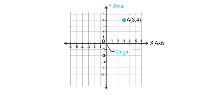
Rene Descartes developed the idea of coordinates coordinates to define the position of a point in a particular space. The reference axes are the basis for defining locations and entities in a Cartesian coordinate coordinate system.
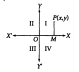
X’OX and Y’OY are two straight lines that act as references. They intersect at right angles, with X’OX being the x-axis and Y’OY being the y-axis. The x-coordinate, also known as abscissa, of point P is the distance of the point from the y-axis (OM), while the y-coordinate or the ordinate is the distance of the point from the x-axis. Together, they are the rectangular or orthogonal coordinates of point P. X, and Y coordinates can be either positive based on their position relative to the reference axes. OY is positive & OY’ is negative. Similarly, OX is positive & OX’ is negative.
Lengths & Distances
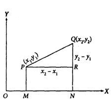
There are two points, P and Q, with Cartesian coordinates (x1, y1) and (x2, y2), respectively. OX and OY are the reference axes. PM and QN are the perpendiculars to the x-axis from points P and Q, respectively. PR is a perpendicular from P to QN.
Now, OM = x1, ON = x2, PM = y1, and, QN = y2. From the figure, we can intuitively say that PR = MN = ON – OM = x2 – x1 and RQ = NQ – NR = NQ – PM = y2 – y1.
Now, taking into the right-angled triangle PRQ, we have 🡪
PQ2 = PR2 + RQ2 = (x2 – x1)2 + (y2 – y1)2
or, PQ = √ [ (x2 – x1)2 + (y2 – y1)2]
Above is the formula for calculating the distance between two points in a coordinate system. Consequentially, we can calculate that the following formula can find the distance of any point from the origin 🡪
√ [ (x)2 + (y)2]
Analytic geometry problems can seem quite convoluted, especially at the advanced & applicational levels. Poor preparation, unclear concepts, and lack of practice can also cause trouble. If you think you could do with some expert geometry homework help, it’s best to pay heed to your intuition and seek professional geometry homework help from a reputed service.
Linear Equations in the Cartesian System
The reference axes in Cartesian space extend to infinity. A point can be placed anywhere between the origin and infinity in both the positive and negative directions, and thus, its coordinates can take on any value. This is where linear algebra overlaps with coordinate geometry.
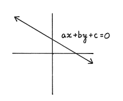
An equation in two variables of the form, ax + by + c = 0, is known as a linear equation as its solutions from straight lines in the rectangular or Cartesian plane.
- Vertical lines in the Cartesian plane run through the x-axis & represent equations of the form x = c, where c is a real number and a constant. All the points or solutions of this equation will have abscissa equal to c.
- Horizontal lines have a fixed ordinate and run through the y-axis. If the ordinate is c, then all points/solutions to the equation have the same value as the ordinate.
- The slope of a line/linear equation is the rate of change in the value of y with respect to the change in the value of x. If a line has the points (x1, y1) and (x2, y2), then the slope is the change in the y-coordinates divided by the change in the x-coordinates.
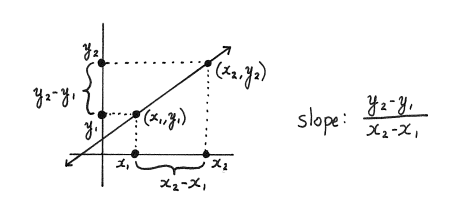
As per the formula mentioned above, if the line above contains the points (-1,4) and (2, -5), then its slope is found to be -3.
- Analytical geometry is used in calculus to represent multivariate equations such as y = ax + b, where a and b are constants. This is a linear equation in the slope-intercept form. b is the y-intercept, while a is the slope of the line.
Having an intercept b means that one solution to this linear equation is the point (0, b). If we put (0, b) in the line equation, then we see that it balances both sides.
b = 0 + b = b
Let’s say we have another point (1, a+b) that’s on the line. So, a+b = a (1) + b, which satisfies the linear equation.
- Now that we have found two points on the line, let’s use them to calculate its slope using the above formula.
We have (0, b) and (1, a+b). According to our formula, we find the slope to be 🡪
(a + b – b) / (1 – 0) = a, same as the expression.
Linear algebra and analytical geometry provide convenient mechanisms for representing any kind of data quantitatively. That’s precisely why both of these topics are the two central foundations of machine learning. Analytical geometry allows for efficient data visualization in any sort of abstract space, enabling accurate, quantitative representation of information in a coordinate system or space.
Interested in learning more about analytical geometry’s applications in data science and machine learning? Then, check out this link. And if you need expert aid with your geometry/data science/machine learning homework and assignments, connect with the homework solvers of Tophomeworkhelper.com right away.
Stay in touch to get more updates & news on Gossips!